Kriging |


|
|
Kriging - it is more flexible method of modeling than a logarithmic interpolation. As well as the logarithmic interpolation, kriging builds a smoothed surface, but in kriging the user can select and customize the modeling function. The surface constructed with use of a Kriging, can, both to touch control points, and to differ in height from control points for smoothing erroneous measurements (see below Nugget). In Kriging for the analysis of existing data distribution there are used the variogram diagrams - the functions calculated by a difference of heights values of pairs of points, that are grouped into lags (groups) by mutual distance between points. Variogram is a measure of the correlation between adjacent points, i.e. characterises how much the neighboring points are similar to each other by value of the modelled characteristic.
g - a variogram for a lag, containing n points (for example, the first lag includes the pairs of of points, distances between which are from 0 to 100 meters, the second lag includes the pairs of points, distances between which are from 100 to 200 meters, etc.); Hi, Hj - value of the modelled characteristic for pair of points i, j; N - number of pairs of points in a lag. Variogram is calculated for each lag and shown on the diagram by points. Over each point of the diagram the number of pairs of points is shown by which value of a variogram was calculated. The horizontal axis of the diagram corresponds to distance between points, and vertical - to value of a variogram. On the basis of these data the researcher needs to choose a function, graph of which one as much as possible is approximated to the initial diagram (to pick a theoretical variogram, modelling an empirical variogram).
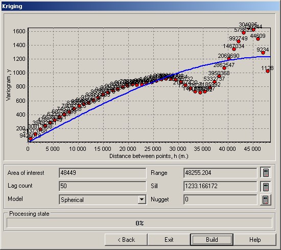
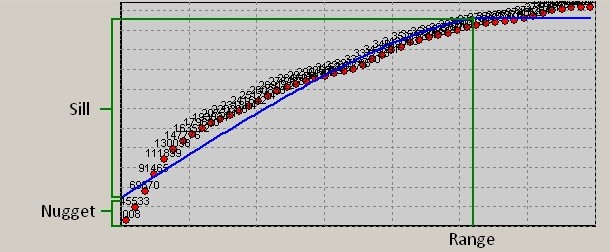
Example of use At initialization of Kriging dialog the following steps are carried out: - points coordinates of the objects having the modelled characteristic are read; - maximal distance between points is determined, which is used for calculation of the size of a lag (number of lags by default is 50); - for each lag the value of empirical variogram is calculated, which is displayed on the diagram by a point with the signature of the number of pairs of the points which have got into a lag; - parameters of the spherical model accepted by default are calculated. The calculated theoretical variogram is displayed in the graph by a blue line.
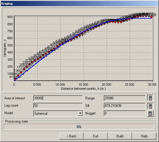
On the presented graph you can see that the value of a variogram increases until the distance between points does not become equal approximately 30000, and then starts to fluctuate. It indicates that the points which are being on distance more 30000, do not correlate with each other. Let's reduce area of interest (analyzed range of distances), having entered 30000 in the field Area of interest.
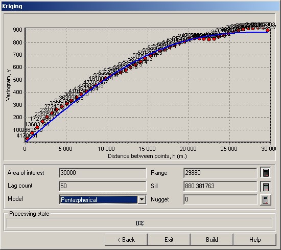
Now we choose from the list of the available models the model, suitable by a form of the diagram of empirical variogram. In this case the most suitable is an exponential model.
For the analysis of separate areas on the diagram it is possible to make its scaling, by selecting the desired area by «a rubber rectangle» top-down. Shift of the increased area concerning all diagram is performed by moving the mouse with the pressed right button. For return to initial scale it is necessary to choose again a rubber rectangle, but this time in the direction bottom-upwards. To operate the form of the diagram of a theoretical variogram it is possible by changing the parameters of the model - radius, a threshold, a nugget (by default these parameters are calculated automatically by points of the empirical variogram).
Range of model's influence is the distance between pairs of points at which the graph of the theoretical variogram is horizontal. Sill (threshold) - value which the variogram model accepts in a point of range of influence (value on axis y) a minus a nugget. The sill and range of modelling function influence curvature of a created surface. Nugget - value of a variogram for pairs of points the distance between which is equal to zero. Theoretically for the same points the value of a variogram should be equal to zero (see the formula). However on infinitesimal distances the difference between measurements often does not tend to zero. This fact is called the nugget effect. Nugget effect can be attributed to measurement errors or the presence of the natural factors, allowing the emergence of the unexpected appearance of emission on distances smaller than the sampling interval (or at the expense of both phenomena). Usually value of a nugget is accepted equal to zero. In this case the height of the constructed surface on the control points is equal to height of these points. In cases where the curve explicitly tries to cross the vertical axis of the graph above zero, it is possible to set nonzero value of a nugget. In this case, the surface will not reach in the height to the control points (the surface will be smoothed in the vicinity of reference points). And smoothing of a control point is greater than more this point differs from neighbours. Therefore use of a nonzero nugget actually allows to execute construction of a surface with an exception of the measurement errors of the modelled characteristic on control points. Any of three parameters can be calculated automatically or entered manually. After parameter change the redraw of the graph is made. Changing manually parameters, it is possible to achieve the best approximation of the model's graph in the desired area. After selecting the parameters of model the launch of building a matrix is performed by pressing the Build button. |